8 Lab 8—Topographic maps
An Introduction to Topographic Maps
by Dr. David Kendrick, Hobart and William Smith Colleges, Geneva, NY, 2005
To use topographic maps, you need to understand several basic map features:
Maps are fundamental geological tools. We use maps to represent a host of information, including rock distribution, water tables, and, most commonly, the shape of the Earth’s surface. Topography is the shape of the Earth’s surface; maps that represent this surface are called topographic maps. Topographic maps depict the Earth’s surface by means of contour lines, or lines of constant elevation.
Goals – your goals in this lab are twofold. 1) Understand how a topographic map represents the Earth’s surface and be able to create and interpret such a map. 2) Solve problems using published topographic maps and your newly discovered map-reading abilities.
Location: Location information identifies the area covered by a map. United States Geological Survey (USGS) maps cover rectangular areas and are identified by a quadrangle name. A state index map shows the locations and names of all the quadrangles in a state and can be used to find the quadrangle that covers a particular area. In addition to quadrangle names, USGS maps are marked with latitude and longitude and other coordinate systems that can be used to locate a map area or feature relative to larger geographic features. The latitude and longitude of California, PA is 40.0625N and 79.8953W, respectively.
Map Scale: Maps are scaled-down representations of an area. This means that the distance between two points on a map corresponds to some true distance on the ground. The ratio of map distance to true distance is the map scale. Most people are familiar with a map’s scale bar. A scale bar is a line or bar of some predetermined map length, 2 cm for example, which is labeled with the corresponding true distance, for example, 2 kilometers. Map scales can also be expressed as a ratio or fraction. Many topographic maps, for instance, have a scale of 1:24,000. This means that one cm on the map equals 24,000 cm on the ground, one foot on the map equals 24,000 feet on the ground, etc. The scale 1:24,000 can also be expressed as a decimal fraction, 1/24000 =0.000041666. While scale bars are handy for a rough approximation of lengths, fractional scales allow precise calculations of lengths. Two equations are particularly useful:
True Distance = (Map Distance) * (Fractional Scale) Map Distance = (True Distance) / (Fractional Scale)
Note: These expressions assume that map and true distances are expressed in the same units! Thus if you measure map distance in cm and calculate true distance, the calculated distance will be in cm. If true distance is in miles and you calculate map distance, the calculated distance will be in miles.
Orientation: Most maps have a North arrow. When the map is oriented so that the North arrow on the map points to north on the Earth, directions on the map are the same as directions on the ground and the map can be used for navigation. In addition to showing true geographic North, USGS maps show magnetic north. In California, the discrepancy is about 9o west; compass needles point to a direction that is 9o west of due North. This “magnetic declination” changes with location—in the western United States, magnetic declinations are east of due North. Besides North arrows, lines of longitude and latitude or other similar coordinate systems can be used to orient a map.
Contour Lines: Contour lines indicate the shape of the land surface, i.e. its topography. A contour line is the map trace of an imaginary line on the ground that has a particular elevation. One way of visualizing such a line is to imagine a shoreline. Bodies of standing water have level upper surfaces, thus their shorelines are traces on the ground surface of that particular elevation. Topographic maps have many contour lines, each adjacent line differing by a constant elevation difference, the contour interval (Figure 1).
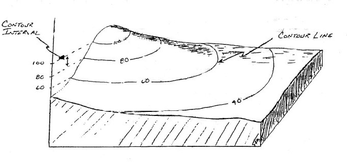
Figure 1: Example of contour lines on a 3-dimensional block diagram.
Contour lines follow some basic rules. If you understand contour lines, you should be able to explain why each of these rules is true:
The closer spaced contour lines are, the steeper the ground surface is.
Contour lines never cross
Contour lines never branch
Contour lines never change elevation
Contour lines never skip (e.g., you can never have the sequence of lines 10, 20, 40 without having 10, 20, 30, 40)
Contour lines always have an up side and a down side (all elevations on one side of the line are higher than the line, all elevations on the other side lower). The up and down side never change along the length of the contour line.
Making a Topographic Profile
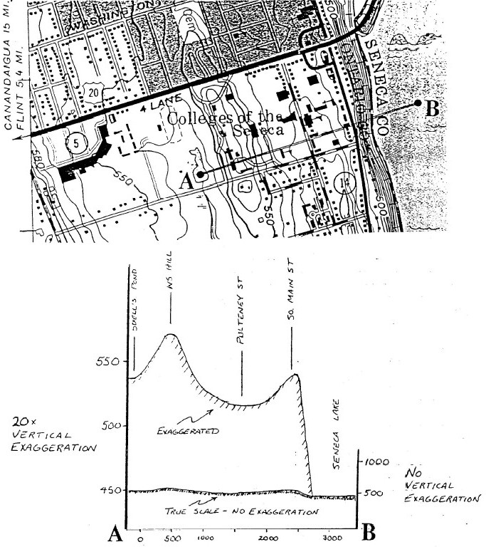
Topographic profiles are scaled drawings depicting the elevation of the land surface along some particular line. Figure 2, for example, is a topographic profile that runs EW through the campus of Hobart & William Smith Colleges in Geneva, NY. A drumlin (a glacial landform that appears as a streamlined hill) is bisected by the profile line.
If the vertical scale of the profile is the same as that of the map, the profile has no vertical exaggeration. Often, however, it is advantageous to use a scale that “stretches” or exaggerates the vertical dimension in order to emphasize topographic features. Figure 2 shows both an unexaggerated and an exaggerated profile. The vertical exaggeration can be calculated from the vertical and horizontal scales. If the horizontal scale is 1:1000 and the vertical scale is 1:50, then the vertical exaggeration is 20 times (20x).
Vertical Exaggeration = (Vertical Scale)/(Horizontal Scale) = (1:50)/(1:1000) = 1000/50 = 20.
Vertical Exaggeration is 20x.
Figure 2: Local area surrounding Hobart and William Smith Colleges, Geneva NY. Note the cross-section line A- B.
LAB 8 – Topographic maps, streams, and drainage basins
Part I: Understanding Topographic Maps
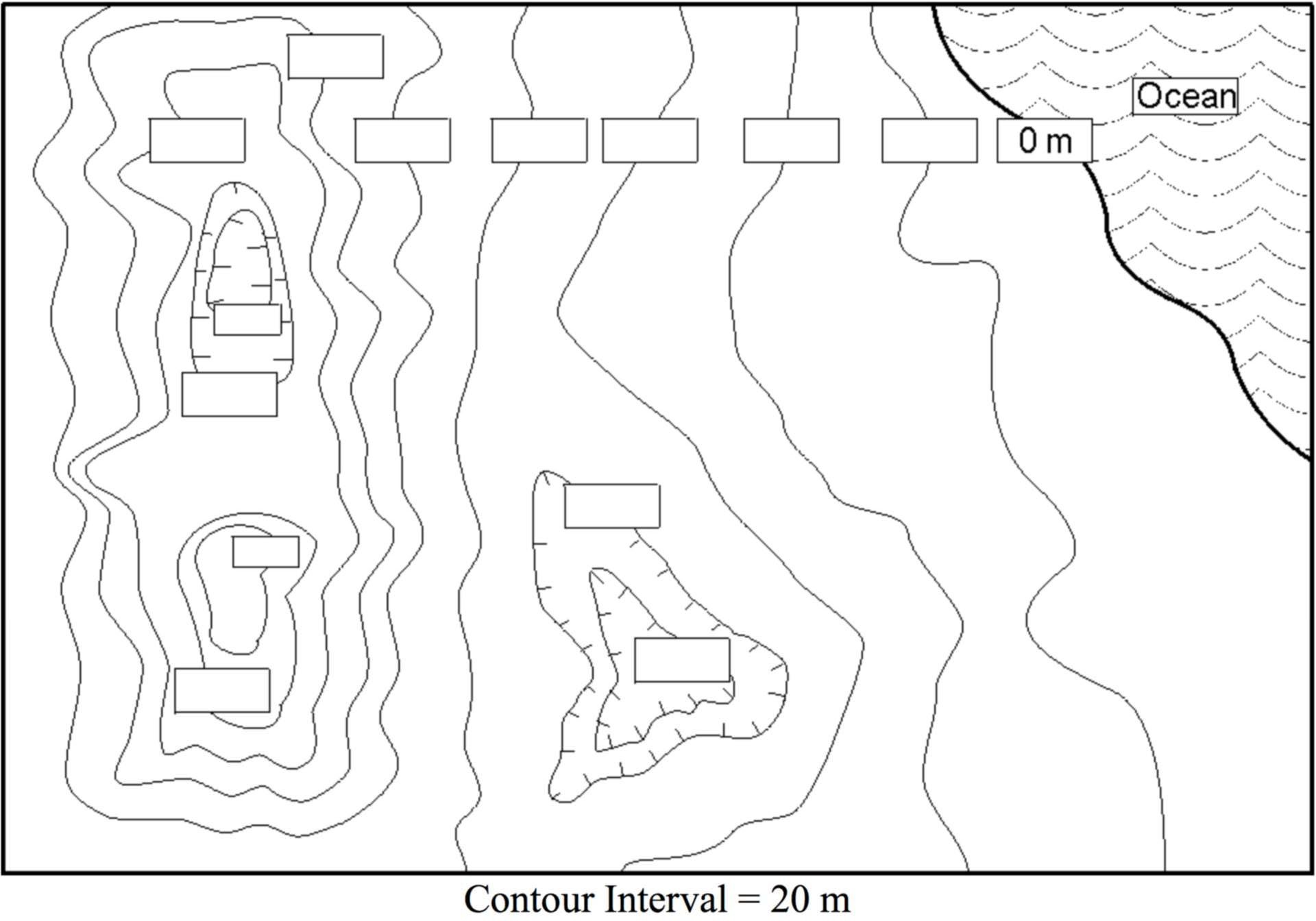
Label the elevation of the contours on the map below. Watch out for depressions with repeated contours!
The shaded relief map below provides elevation measurements (in feet) across the island of Hawaii, an active volcanic island with two large peaks, Mauna Kea and Mauna Loa. Using a 3000 ft contour interval, draw and label the contour lines across the island. Sea level elevation = 0 ft. Don’t forget about the rule of V’s! Estimate the elevation of location X by interpolating between the contour lines.
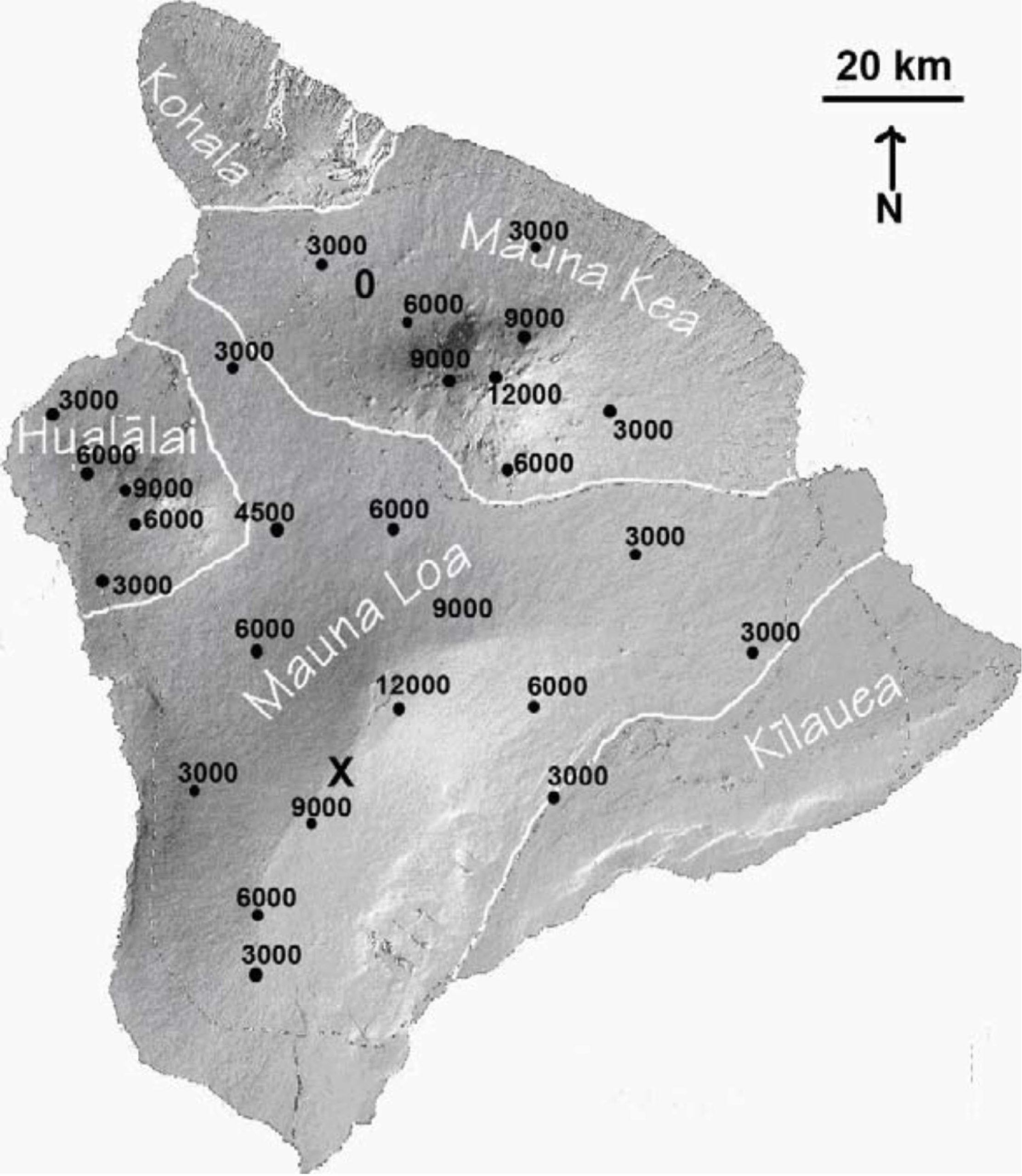 X =ft
X =ft
Using the topographic map below, construct a topographic profile from A to A’. To easily measure distance, fold your paper along the dotted line below the graph and line the crease up with the A to A’ profile line (or use a ruler). Grey shaded areas are rivers.
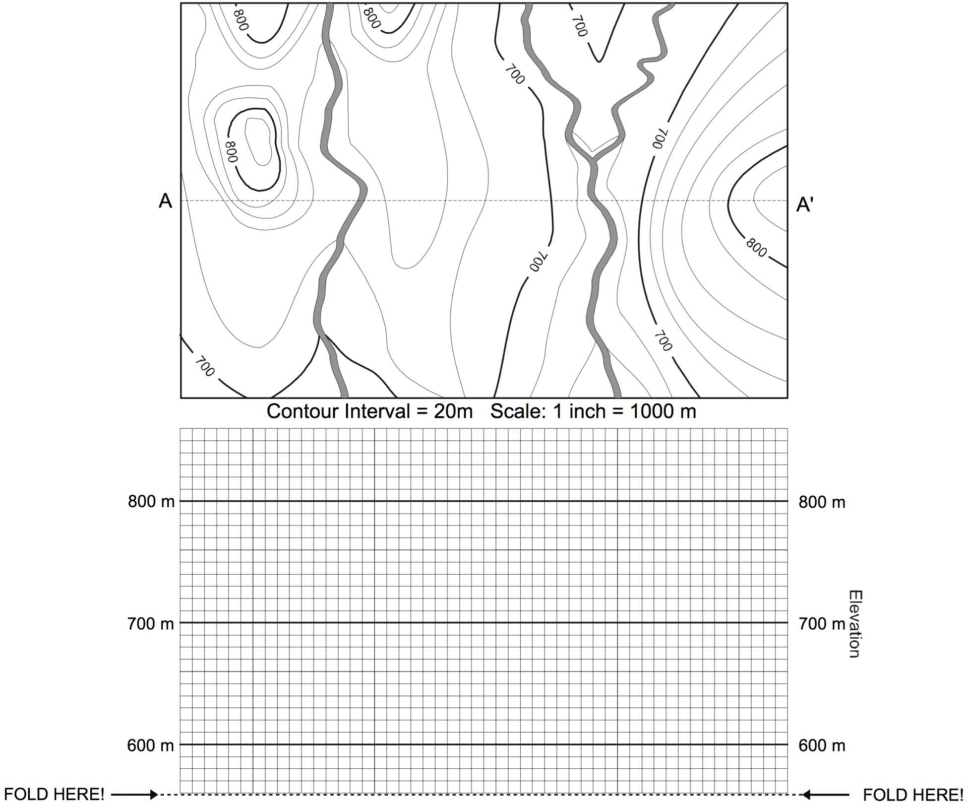
On the profile you just created:
What is the horizontal scale in meters/inch?
What is the vertical scale in meters/inch?
What is the vertical exaggeration?
Part II: USGS Topographic Maps
For this section, examine one of the topographic maps provided. All of the information in this section is written somewhere on the map so it should be relatively easy to find.
What is the name of this quadrangle?
What part of which state is this quadrangle in?
Is this a 7 1/2 or a 15 minute quadrangle?
What is the difference in area between a 7 1/2 and a 15 minute quadrangle?
What is the ratio scale of this map?
How many meters in real life does 1 cm on the map equal?
1 cm on the map =____________meters in real life
What is the magnetic declination in the area of this map?
If you wanted to hike eastward past the limit of this map, which quadrangle would you need a map of?
What is the contour interval of this map?
What is the INDEX CONTOUR interval of this map?
Where, in general, is the highest elevation in this quadrangle? What is the elevation there?
Where, in general, is the lowest elevation in this quadrangle? What is the elevation there?
What is the total relief of the map?
Part III: Using topographic maps to measure streams and drainage basins
Locate Map 1 and find its location on the location map page. You are looking at two very small streams in the Mt. Airy region of Cincinnati. These streams are not drawn on the map, but their basins should be labeled 1 and 2.
What larger stream do these two basins contribute to? What river does that stream enter? Where does this water end up when it reaches sea level?
Draw an arrow indicating which direction the west fork of Mill Creek is flowing here.
Using the contour lines a guide, draw in the stream network in each of the two basins, directly on the map. Follow each stream to where it joins the west fork of Mill Creek.
On the map, draw the drainage divides for each of these basins, again using the contours as a guide.
On the graph paper below, construct a longitudinal stream profile for the main stem (longest) streams in basin 1 and basin 2.
You will need to plot elevation on the vertical axis vs. stream distance on the horizontal axis. The contour crossings are good places to measure these values.
Your profiles should both begin where the west fork of Mill Creek exits the map and extend upstream to the drainage divide in each basin.
You will need to measure distance along the stream with a ruler, and to convert map units to real-world distance. Be sure to label your axes, including units!

On the profile you just created:
What is the horizontal scale in meters/inch?
What is the vertical scale in meters/inch?
What is the vertical exaggeration?
What differences exist between the elevation profiles of two streams?
Are there any changes in slope (stream gradient) visible along the profiles? Describe them.
What is the steepest stream gradient present in basin 1? At what elevation is it found?
What is the steepest stream gradient present in basin 2? At what elevation is it found?
Using the drainage basins you delineated, measure the drainage area contributing to each stream above where it joins the west fork of Mill Creek. You can use the grid on the map to estimate the area of the basin (note the grid spacing by comparison to the map scale).
Area of basin 1:m2
Area of basin 2:m2
Assuming the average rainfall is the same for both drainage basins (which it should be, as they are very close together!), which one would you expect to have a larger stream in it?
Given your answer to the previous question, and what you know about streams, develop an explanation for the difference in stream gradient between the two basins.
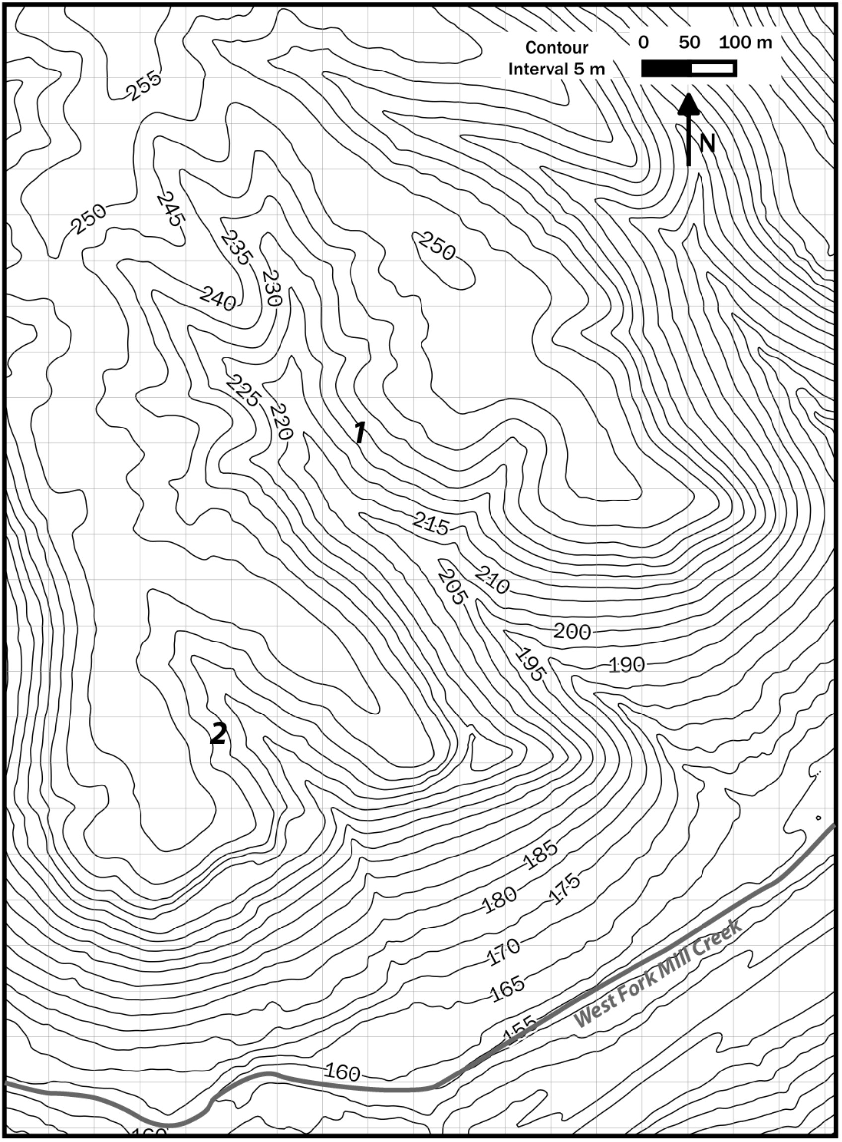
Map 1. Small creeks in Mt. Airy Forest, Cincinnati.
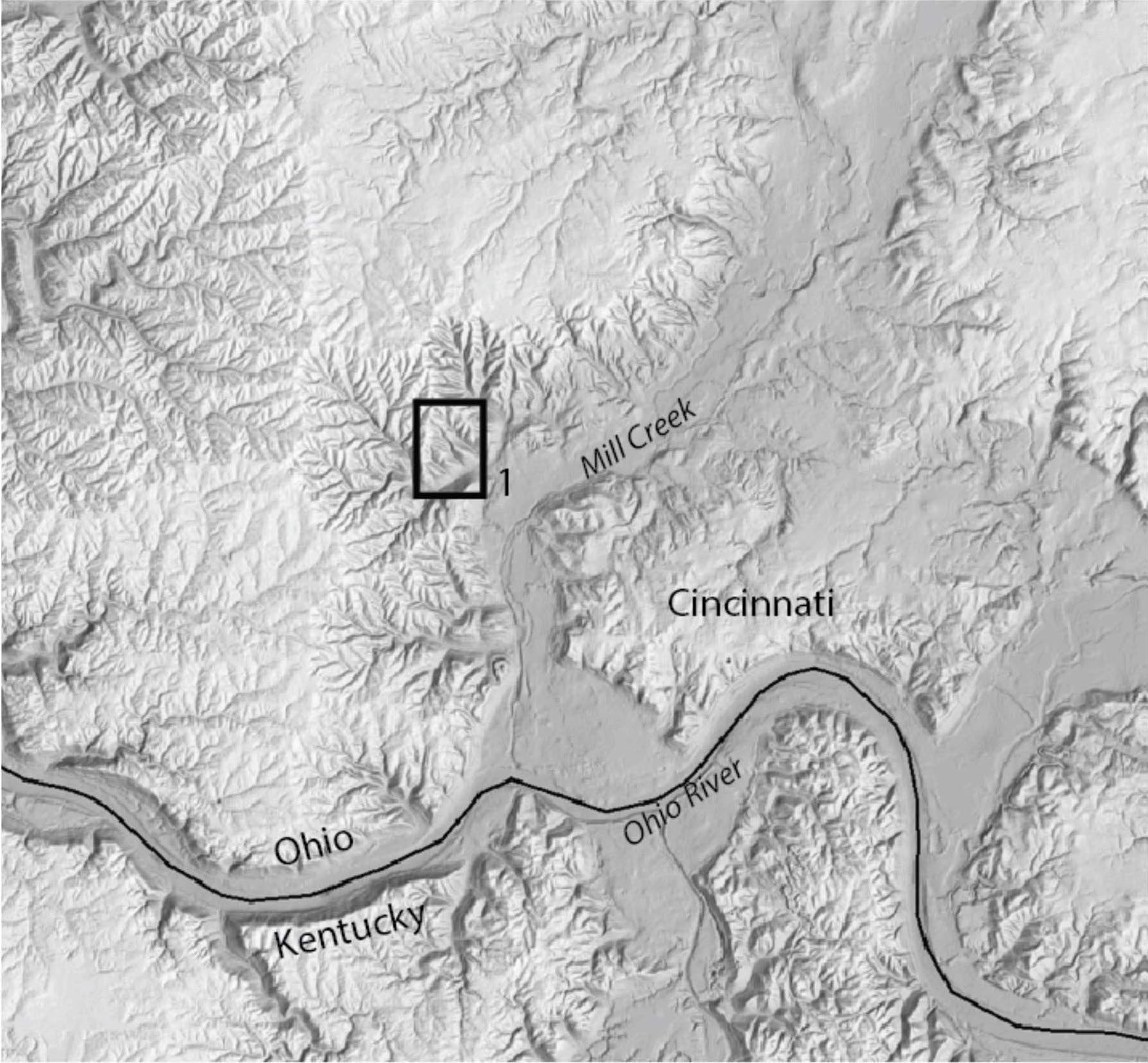 Location of Map 1.
