14 Lab 14—Glaciers

Objectives: Develop a deeper understanding of glacial motion by conducting a physical experiment emulating alpine glaciation.

Outcomes: By the end of the activity, you will be able to 1) explain how ice flows within an alpine glacier, 2) quantitatively describe ice motion and glacial metrics (e.g. velocity, discharge), 3) begin to discuss how alpine glaciers respond to changing environmental conditions, and 4) evaluate the successes and shortcomings of using physical models to understand glacier dynamics.

Activity Instructions

Please make sure that you read the activity instructions fully before you begin. There are questions at the end. Be sure to design your experiment in such a way that you will be able to answer those questions. The materials for your physical model have been set up prior to class for you.

Equipment list: Glacier goo, ruler, PVC pipe, pencil, timer, calculator and stack of books.

You will first need to mix your glacier goo, following the directions provided in the image above.

For your glacier advance calculations, you are required to measure the velocity and discharge of your glacier over a two-minute period. Discuss with your group the best way of calculating these metrics. The following 3 equations may prove useful:

where:

where:

where:

**we will assume that the glacier fills the full half of the PVC pipe. Think about how this may bias the calculations you will make during the lab**

Using your physical model, measure the velocity and discharge of your glacier over 2 minutes. Record your results in the table blow. The column names may offer some clues about what measurements you will need to complete this exercise. ** note the units!! **

Answer these questions concerning your experiment:

1. How does velocity vary across the glacial valley?
2. How does does velocity vary with depth?
3. What observations did you make to conclude this?
4. What is influencing the glacier’s velocity?
5. What might increase the simulated glacier’s velocity?
6. What might decrease its velocity?
7. If the PVC pipe was lined with a different substrate (e.g., sandpaper) how might the velocity and discharge of the glacier change?
8. How well does this physical model emulate the real-world system?
9. What is realistic/unrealistic about the model?
10. What aspects of the glacial system does this model capture?
11. What important aspects of a real-world glacier system were not modeled by your experiment?

Look at the Glacial Map of Ohio and read the information page below about the glacial deposits of Ohio.

For questions #1-5, define the following terms from the map legend and describe how they relate to a glacier or ice sheet. You may use your lab manual, Wikipedia, or your classmates for help.

1. Moraine:
2. Esker:
3. Outwash:
4. Peat:
5. Colluvium:
6. Find the oldest deposits on the map. Where are they?
7. How old are the oldest deposits?
8. To which glacial stage do the oldest deposits belong?
9. Draw a line on the map outlining the southern extent of Wisconsinan stage glacial deposits. This is where the terminus of the ice sheet was located about 20,000 years ago.
10. Was the Illinoian stage ice sheet larger or smaller than the Wisconsinan stage ice sheet?
11. What evidence did you use to answer question #10?
12. List several reasons why the ice sheet may have been larger during one stage than during another.
13. On the map, find the Wisconsinan-stage ridge moraines and number them (1,2,3,…) from oldest to youngest, starting with 1 as the oldest moraine.
14. What does this sequence of moraines that you labeled for question #13 represent?

STATE OF OHIO •DEPARTMENT OF NATURAL RESOURCES•DIVISION OF GEOLOGICAL SURVEY

GLACIAL MAP OF OHIO

GLACIAL DEPOSITS OF OHIO

Although difficult to imagine, Ohio has at various times in the recent geologic past (within the last 1.6 million years) had three-quarters of its surface covered by vast sheets of ice perhaps as much as 1 mile thick. This period of geologic history is referred to as the Pleistocene Epoch or, more commonly, the Ice Age, although there is abundant evidence that Earth has experienced numerous other “ice ages” throughout its 4.6 billion years of existence.

Ice Age glaciers invading Ohio formed in central Canada in response to climatic conditions that allowed massive buildups of ice. Because of their great thickness, these ice masses flowed under their own weight and ultimately moved south as far as northern Kentucky. Oxygen-isotope analysis of deep-sea sediments indicates that more than a dozen glaciations occurred during the Pleistocene. Portions of Ohio were covered by the last two glaciations, known as the Wisconsinan (the most recent) and the Illinoian (older), and by an undetermined number of pre-Illinoian glaciations.

Because each major advance covered deposits left by the previous ice sheets, pre- Illinoian deposits are exposed only in extreme southwestern Ohio in the vicinity of Cincinnati. Although the Illinoian ice sheet covered the largest area of Ohio, its deposits are at the surface only in a narrow band from Cincinnati northeast to the Ohio- Pennsylvania border. Most features shown on the map of glacial deposits of Ohio are the result of the most re- cent or Wisconsinan-age glaciers.

The material left by the ice sheets consists of mixtures of clay, sand, gravel, and boulders in various types of deposits of different modes of origin. Rock debris carried along by the glacier was deposited in two principal fashions, either directly by the ice or by meltwater from the glacier. Some material reaching the ice front was carried away by streams of meltwater to form outwash deposits. Material deposited by water on and under the surface of the glacier itself formed features called kames and eskers, which are recognized by characteristic shapes and composition. A distinctive characteristic of glacial sediments that have been deposited by water is that the material was sorted by the water that carried it. Thus, outwash, kame, and esker deposits normally consist of sand and gravel. The large boulder-size particles were left behind and the smaller clay-size particles were carried far away, leaving the intermediate gravel- and sand-size material along the stream courses.

Material deposited directly from the ice was not sorted and ranges from clay to boulders. Some of the debris was deposited as ridges parallel to the edge of the glacier, forming terminal or end moraines, which mark the position of the ice when it paused for a period of time, possibly a few hundred years. When the entire ice sheet receded because of melting, much of the ground-up rock material still held in the ice was deposited on the surface as ground moraine. The oldest morainic deposits in Ohio are of Illinoian and pre-Illinoian age. Erosion has significantly reduced these deposits along the glacial boundary, leaving only isolated remnants that have been mapped as dissected ground moraine and hummocky moraine.

Many glacial lakes were formed in Ohio during the Ice Age. Lake deposits are primarily fine-grained clay- and silt-size sediments. The most extensive area of lake deposits is in northern Ohio bordering Lake Erie. These deposits, and adjacent areas of wave-planed ground moraine, are the result of sedimentation and erosion by large lakes that occupied the Erie basin as Wisconsinan-age ice retreated into Canada. Other lake deposits accumulated in stream valleys whose outlets were temporarily dammed by ice or outwash. Many outwash-dammed lake deposits are present in southeastern Ohio far beyond the glacial boundary. Peat deposits are associated with many lake deposits and formed through the accumulation of partially decayed aquatic vegetation in oxygen-depleted, stagnant water.

The term glacial drift commonly is used to refer to any material deposited directly (e.g., ground moraine) or indirectly (e.g., outwash) by a glacier. Because the ice that invaded Ohio came from Canada, it carried in many rock types not found in Ohio. Pebbles, cobbles, and boulders of these foreign rock types are called erratics. Rock collecting in areas of glacial drift may yield granite, gneiss, trace quantities of gold, and very rarely, diamonds. Most rocks found in glacial deposits, however, are types native to Ohio.

Certain deposits left behind by the ice are of economic importance, particularly sand and gravel, clay, and peat. Sand and gravel that have been sorted by meltwater generally occur as kames or eskers or as outwash along major drainageways. Sand and gravel are vital to Ohio’s construction industry. Futhermore, outwash deposits are among the state’s most productive sources of ground water. Glacial clay is used in cement and for common clay products (particularly brick). The minor quantities of peat produced in the state are used mainly for mulch and soil conditioning.

Introduction: Glaciers are ephemeral climate-related features that dramatically imprint the shape of the landscape over time. This investigation examines the historical changes to Grinnell Glacier in Glacier National Park, Montana (Fig. 14.2). Grinnell Glacier is one of the largest remaining glaciers in the park, even though it is less than a square mile in area. In this investigation, we’ll estimate how long it will be before there are no longer glaciers in Glacier National Park, based on historical records.

Historical Field Mapping: First measurements of glaciers in Glacier National Park were conducted as part of topographic field mapping in 1900. From the early 1900’s to the 1960’s, several scientists working with the National Park Service created a photographic archive of glaciers, with re-surveying on a regular basis throughout the 1900’s. See the attached map (Fig. 14.1) showing the position of the glacial front historically during the early and mid-1900’s (The map is from U. S. Geological Survey Professional Paper 1180: Grinnell and Sperry Glaciers, Glacier National Park, Montana: a Record of Vanishing Ice, published by the USGS in 1980).

Part I: Initial Observations and Predictions

Consider the map in Figure 4.1, showing the areas Grinnell Glacier covered in 1850, 1937, 1968, and 1993, and the glacial front positions for 1887, 1937, 1946, 1960, and 1968. Based on only this evidence, answer the following questions:

1. Has this glacier been advancing or retreating over time?
2. What factors control glacial advance and retreat?
3. Approximately how many years do you think it will be until Grinnell Glacier is completely melted?
4. How did you produce your estimate?

Part II: Data collection

Divide into four teams. Each group will choose a year (1850, 1937, 1968, or 1993). Using the map in Figure 14.1, note the outline of the extent of Grinnell Glacier for your year. Then carefully cut out your glacier outline. Trace it onto the graph paper provided. Then count the number of squares of graph paper contained within your traced outline. Count every full square and any square that is more than halfway in your traced outline. The total should be very close to the surface area of Grinnell Glacier that year, in “squares.” But how big is each square of your graph paper? Compare the squares of the graph paper to the map scale. Convert your counted area to a more practical unit of measurement. Determine the following:

1. Year of glacial front used in analysis: _____________
2. Total number of graph squares in glacial area: ___________
3. Map scale of Figure 2:        1 inch on map = ______________ meters on ground
4. 1 square inch on map = ______________ square meters on the ground
5. Number of graph squares per square inch = ________________
6. Number of square meters per graph square = ____________________
7. Total scaled area of active glacier for your year in square meters: ___________________
8. Total scaled area of active glacier for your year in square kilometers: __________________
9. Distance of glacial front in your year, from upper most elevation of ice (m) ______________
10. Distance of glacial front in your year, from upper most elevation of ice (km) ______________

Sharing data with other teams, complete this table.

Part III: Analysis

Using Excel, or another favorite software package, or hand graphing techniques, create the following graphs:

1. Active Glacier Area (Y-axis) vs. Year (X-axis)
2. Distance of Front (Y-axis) vs. Year (X-axis)

Part V: Interpretation

Now, it’s time to revisit the question posed in Part I:

1. Approximately how many years do you think it will be until Grinnell Glacier is completely melted?
2. In the discussion of your data, provide a linkage between your observations at Grinnell Glacier, and the historic global atmospheric temperature data depicted in the graph on Figure 14.3.
3. How do your results fit with the context of global climate change and possible causes for historic glacial retreat?
4. What are long-term implications from glacial analysis at Glacier National Park, Montana?

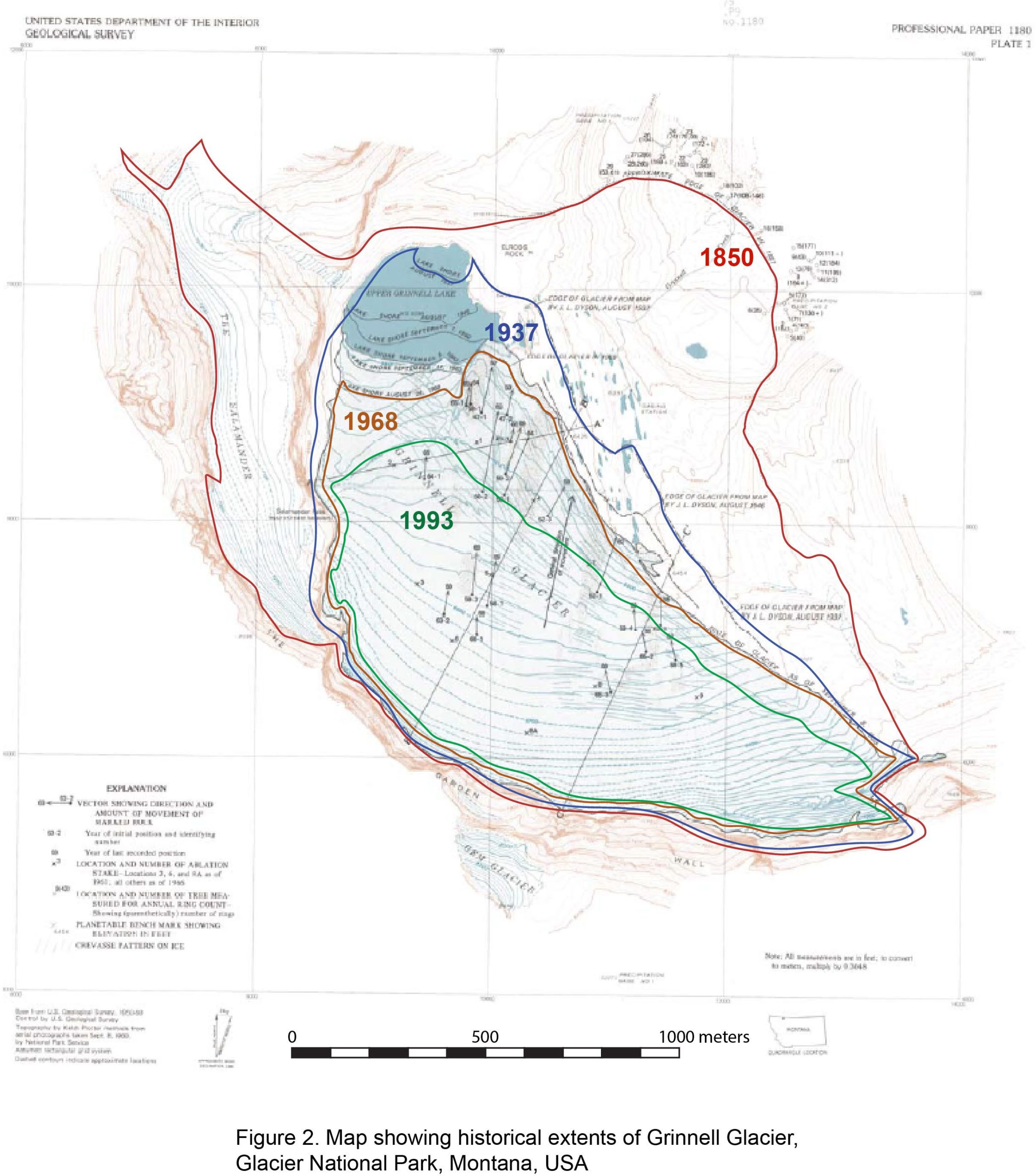
Figure 14.1. Map showing historical extents of Grinnell Glacier, Glacier National Park, Montana, USA.

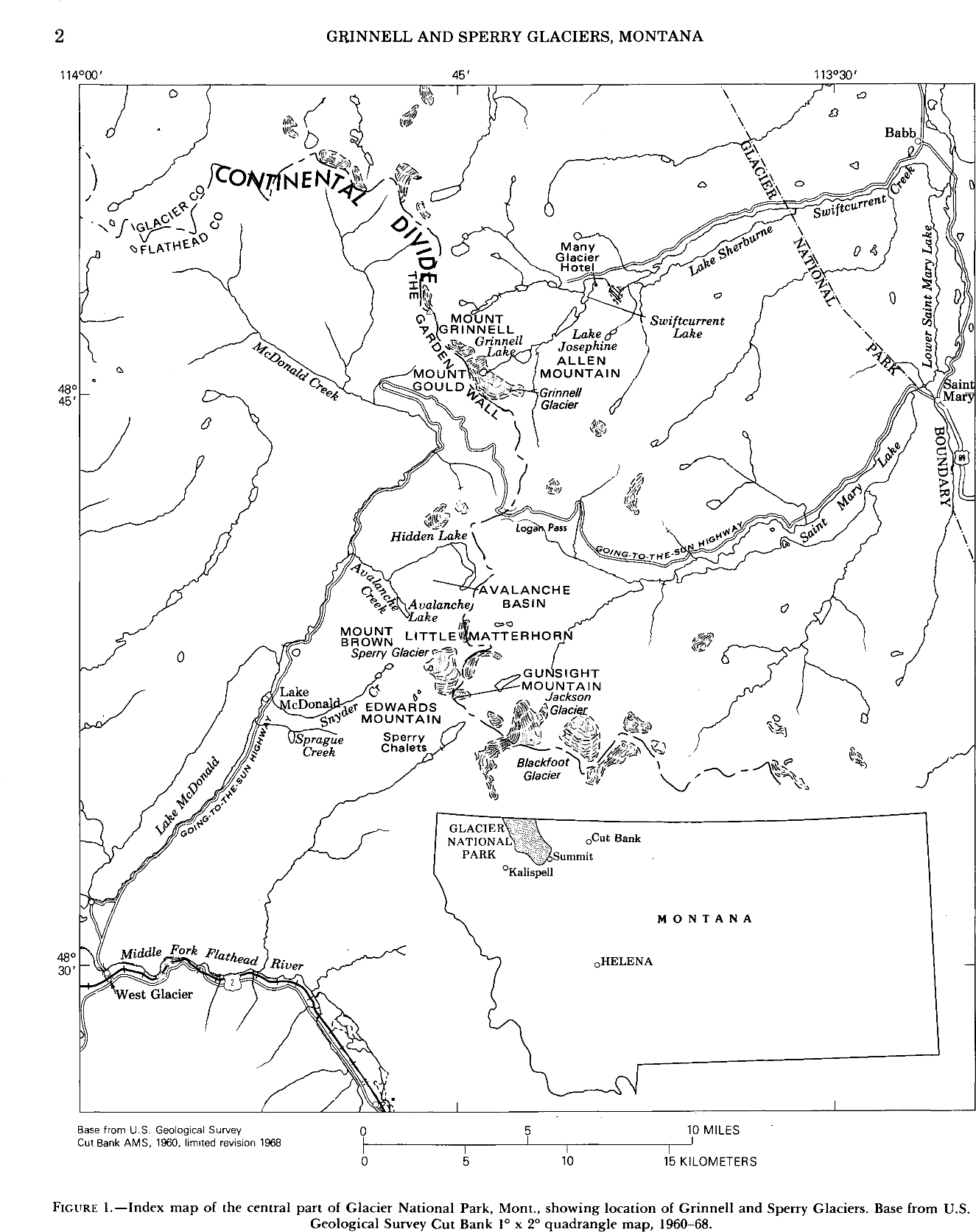
Figure 14.2. Index map of the central part of Glacier National Park, Montana, showing location of Grinnell Glacier, from Johnson, A, 1980: Grinnell and Sperry Glaciers, Glacier National Park, Montana: A record of vanishing ice. No. 1180. US Government Printing Office.

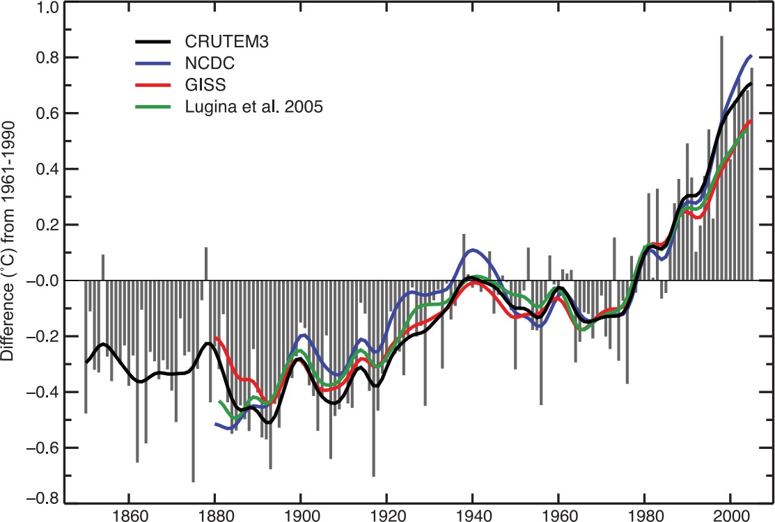
Figure 14.3. Annual anomalies of global land-surface air temperature (°C), 1850 to 2005, relative to the 1961 to 1990 mean for CRUTEM3 updated from Brohan et al. (2006). The smooth curves show decadal variations (see Appendix 3.A). The black curve from CRUTEM3 is compared with those from NCDC (Smith and Reynolds, 2005; blue), GISS (Hansen et al., 2001; red) and Lugina et al. (2005; green) from Trenberth, K.E., P.D. Jones, P. Ambenje, R. Bojariu, D. Easterling, A. Klein Tank, D. Parker, F. Rahimzadeh, J.A. Renwick, M. Rusticucci, B. Soden and P. Zhai, 2007: Observations: Surface and Atmospheric Climate Change. In: Climate Change 2007: The Physical Science Basis. Contribution of Working Group I to the Fourth Assessment Report of the Intergovernmental Panel on Climate Change [Solomon, S., D. Qin, M. Manning, Z. Chen, M. Marquis, K.B. Averyt, M. Tignor and H.L. Miller (eds.)]. Cambridge University Press, Cambridge, United Kingdom and New York, NY, USA.

References:

Cesta, Jason and Elizabeth Orr (2018) “Laboratory 1: An introduction to glacial dynamics.”
“Glacial Map of Ohio.” 1:2000000. Ohio Department of Natural Resources, Division of Geological Survey, 2005. https://ohiodnr.gov/wps/wcm/connect/gov/e1c431e3-3ff4-4eb1-812f-7d0802127b81/Glacial+Map+of+Ohio.pdf?MOD=AJPERES&CVID=ne.WIDF; last access: 2022-10-13.
“Glaciers” National Snow & Ice Data Center. https://nsidc.org/learn/parts-cryosphere/glaciers; last access: 2022-10-13.
Ormand, Carol, 2010, “Investigation: When will there no longer be glaciers in Glacier National Park?” https://serc.carleton.edu/quantskills/activities/glacial_retreat.html; last access: 2021-11-23.
Ward, Dylan (2017) “In class exercise: Glacial geology of Ohio.”