11 Lab 11—Geophysical Field Methods
What is Geophysics?
Geophysics is the study of the physical processes and physical properties of the Earth and its surrounding space environment, and the use of quantitative methods for their analysis. Data that is gathered relies upon the interactions of Earth’s materials with physical fields:
Density, electrical resistivity, electrical fields and radioactivity of rocks;
Velocity of sound waves transmitted through the ground;
Changes in gravity and magnetic fields of the Earth; or
Reflection of radio signals from rocks near the Earth’s surface.
Geophysicists use one or more of these measurements to find oil, natural gas, potash, coal, iron, copper and many other minerals. In addition, the properties are used to identify environmental hazards and evaluate areas for dams or building construction sites.
Definitions given by the Environmental and Engineering Geophysical Society (n.d.) are as follows:
Geophysics is: The subsurface site characterization of the geology, geological structure, groundwater, contamination, and human artifacts beneath the Earth’s surface, based on the lateral and vertical mapping of physical property variations that are remotely sensed using non-invasive technologies. Many of these technologies are traditionally used for exploration of economic materials such as groundwater, metals, and hydrocarbons.
Geophysics is: The non-invasive investigation of subsurface conditions in the Earth through measuring, analyzing and interpreting physical fields at the surface. Some studies are used to determine what is directly below the surface (the upper meter or so); other investigations extend to depths of 10’s of meters or more.
Both of these definitions have a common component, namely that geophysics represents a class of subsurface investigations that are non-invasive (i.e. that do not require excavation or direct access to the sub-surface). The exceptions are borehole geophysical methods that expand the use of holes already drilled to access the subsurface on a very localized basis.
In addition, Definition 1. focuses on the key targets of interest (i.e. geology, geological structure, etc.) – a key consideration in understanding the realm of Environmental and Engineering Geophysics.
Definition 2. underscores the near surface aspect (i.e. in contrast to other geophysical applications, such as petroleum or mineral exploration, this type of problem solving deals with shallow depths that are most significant in terms of the lives, work and activities of the earth’s human population.)
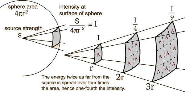
Figure 11.1. Illustration of the general behavior of fields obeying an inverse-square law (from Nave, n.d.).
Geophysical studies are premised upon the interactions of Earth’s materials with physical fields. These fields obey the inverse-square law of physics (Fig. 11.1). “Any point source which spreads its influence equally in all directions without a limit to its range will obey the inverse square law. This comes from strictly geometrical considerations. The intensity of the influence at any given radius r is the source strength divided by the area of the sphere. Being strictly geometric in its origin, the inverse square law applies to diverse phenomena. Point sources of gravitational force, electric field, light, sound or radiation obey the inverse square law” (Nave, n.d.).
Examples of five different fields used in geophysics than can be described using inverse-square laws include
- Newton’s law of universal gravitation, Fg=(Gm1m2)/r2, where Fg is the gravitational force, G is the gravitational constant, m1 and m2 are the masses of two objects, and r is the distance between them;
- sound, applicable to geophysics in the form of seismic waves, I = W/(4πr2), where W is the power of the sound source and I is the intensity in decibels at a distance of r from that source;
- Coulomb’s law for the electrical force between two charged particles (with charges of q1 and q2), Fe=kq1q2/r2, where k is a constant;
- radar, Pr=(PtGtArσF)/[(4πrr2)(4πrt2)], since radar calculations need to account for the emitted waves and the received waves, r2 shows up twice in the denominator;
- and the one that applies directly to this week’s lab, magnetism, Fm=μp1p2/r2, where μ is a constant, and p1 and p2 are the strength of two independent magnetic poles.
Near-surface geophysical surveys are conducted, as their name implies, to characterize the nature of the subsurface just below the surface. These include ground-penetrating radar surveys, shallow seismic surveys, electrical resistivity surveys, and the kind you are going to do in the following activity: magnetometry surveys.
Exercises
Geophysics Activity—Magnetometry at home: a hands-on survey with your smartphone (Bank, 2021)
Geophysical surveys, including magnetometry, take advantage of contrasts in physical properties between targets in the subsurface and the material surrounding them. These property contrasts allow us to measure variations in some quantity at or above the surface and then interpret what may be present in the subsurface. My team has used magnetometry for example to locate buried firearms1 or to determine depth to bedrock2 or for a historical archaeology project3.
What are other (maybe more common) targets for magnetometry? Do an internet search, or check a geophysics textbook, to find an interesting discovery that was made using magnetometry and share it on the discussion board.
This exercise will allow you to think through the process of a magnetic survey; however, it was designed during the COVID-19 pandemic so assumes minimal ability to move about. To accommodate your particular situation (are you able or allowed to leave your home? can you run a survey in the yard or the driveway if you live in a house? can you access a park?) you are asked to use a known magnetic target (a fridge magnet, a car, a fence, a lamp post) and measure its magnetic effect. The main goal of this exercise is to have you perform and document a survey. You will be completing a worksheet and can look at an example we created from a tabletop survey (Toronto is under lockdown as I am preparing this). In a follow-up exercise you are given magnetic data that was collected in a field survey and will be analysing that by comparing it to a model you create. If you are lucky and have access to a backyard with a known buried target (for example a near-surface buried metal pipe) you can follow this exercise by running a survey there.
Learning outcomes:
This exercise will allow you to
- select a target and design a magnetic survey,
- collect field data (with field being very broadly defined) using a free app,
- document your survey,
- graph the data you obtained,
- complete a simple quantitative analysis, and
- communicate your findings.
1 Deng, E. A., K. O. Doro, and C-G Bank, 2020. Suitability of magnetometry to detect clandestine buried firearms from a controlled field site and numerical modeling, Forensic Science International, 314: 110396, https://doi.org/10.1016/j.forsciint.2020.110396
2 Papadimitrios, K., C.-G. Bank, S. Walker, and M. Chazan, 2019. Paleotopography of a Paleolithic landscape at Bestwood 1, South Africa, from ground-penetrating radar and magnetometry, South African Journal of Science, 115(1/2), Art. #4793, 7 pg., https://doi.org/10.17159/sajs.2019/4793
3 Wadsworth, W., C.-G. Bank, K. Patton, and D. Doroszenko, 2020. Forgotten Souls of the Dawn Settlement Project: A geophysical exploration of unmarked graves in Southwestern Ontario. Historical Archaeology, Vol 54, https://doi.org/10.1007/s41636-020-00251-7
Preparation

Figure 1: Screenshot of “Physics Toolbox Sensor Suite” app
Download and install the free “physics toolbox” app, available for both Android and iOS devices (see https://www.vieyrasoftware.net/ for info and link to download). For this exercise you will just need the “Physics Toolbox Magnetometer” that you can download individually. You may be surprised how many sensors are included in your device: accelerometer, sound detector, barometer, GPS… though not all tools may be supported (e.g., my iPad cannot run the proximeter).
After download, start the app. You should see a screen like the one in figure 1, the different colours mark the 3 components (x, y, z) and the total value of the magnetic field. By pressing the red button, you can record the measurements and save them as a spreadsheet (.csv) file.
Print a copy of this worksheet (this would resemble working with a field notebook). You may also complete it on your computer device (if you can take the computer to your survey location and have a stylus, or you can scan and insert any drawings).
And here is a question to start you off:
What feature or app on your smartphone may make use of the built-in magnetic sensor? your answer:
Brief background
Magnetic surveys allow us to locate buried objects or features if they distort the Earth’s magnetic field that we measure at the surface or from an aerial vehicle. These objects can be either a permanent magnet or a material that acts like a magnet because it is within a magnetic field. A magnet can both attract and repel another magnet, and the direction of force around a magnet changes. We describe a magnet as a dipole and find that the force does not point towards the magnet and that it drops off with the cube of the distance if we move in a straight line away from the dipole. This exercise allows you to confirm this relationship.
Variations in the Earth’s magnetic field that are caused by a buried magnetic object are called anomalies. Because of the dipole nature of magnets most anomalies are paired (that is a positive, larger than the ambient field, and a negative anomaly arise from the same target), and anomalies for similar objects will look different depending on the latitude where we measure them. This exercise does not explore such relationships, because some of you may have to run the experiment in a very “noisy” environment (I live in a downtown apartment building), and geophysicists use more sensitive magnetometers than that in your smartphone because they need to measure very small anomalies. If you want to learn more about magnetic surveys in geophysics check out http://appliedgeophysics.berkeley.edu/magnetic/index.html (Berkeley Course in Applied Geophysics) and/or https://www.eoas.ubc.ca/ubcgif/iag/methods/meth_3/index.htm (UBC Applied Geophysics Learning Objects), the latter includes some self-test questions.
A few background questions linked to magnetic surveying in geophysics:
What is the difference between remanent and induced magnetization? How could you distinguish between the two on a magnetic map?
Why do we need to know the latitude of our survey to make sense of the data?
What are key processing steps typically applied before interpreting the data?
What are key advantages and shortcomings of magnetic surveys?
Can magnetometry surveys be used to find buried objects on other planetary bodies? Please share your thoughts on the discussion board. Answers to these questions are not crucial to complete this exercise. Therefore, you may think about them afterwards, especially if you are doing this exercise as part of an introductory geophysics course or if it will be followed by a field survey.
Task 1: What is the objective of your survey?
Most decisions (where to go, what equipment to take, how to set up, how large a survey) hinge on this question. In this exercise we ask you to collect magnetic data along a survey line. If you can go outside find something (a parked vehicle, a fence, . . .) and check with the magnetometer app that values are changing. Note that if you turn around on the spot, or tilt your device readings probably will change, so make sure you hold it steady while you explore for a target.
Briefly state your survey objective:
Task 2: General considerations
It is a good idea to consider some general questions: what are the date and time of day? Who are you with? If you are outside, what is the current weather? What are the ground conditions (did it rain, covered in snow, muddy)? Anything else noteworthy before you start?
Task 3: Documenting your location
Your need to communicate to another person the location (and layout) of your experiment as accurately as possible so they could exactly recreate your experiment.
3a) Handheld devices can provide your location. To find it on either iOS Maps or Google maps open the app, hold a finger on the screen at your location which “drops a pin” and scroll down (in Google maps) or tap “My Location” (in iOS) to view your latitude and longitude.
What are your GPS coordinates, and what did you use to determine them?
3b) Describe your exact location in point form. If you are outside look around, are there any remarkable features (a corner in a fence, a large rock, an odd-shaped tree, buildings nearby) that can help someone else find the exact spot where you are?
3c) Are there any features that may impact your survey (power lines, parked equipment, buildings, mountain, canyon, closeness to industrial operation, airport)?
3d) Draw a map sketch of your location. This should include the features you noticed in 1b. Also include a scale and the North direction. Make your sketch large enough so you can add the layout of your experiment afterwards.
You now have documented your location in three ways: by GPS coordinates, in words, and by a sketch. This may seem redundant but consider that these are complementary and all helpful for someone else to exactly recreate your survey.
Task 4: Setting up your survey
Typically, in magnetometry the deeper the buried object is, the larger an area at the surface will be affected (ie. measurements deviate from the background reading, that is called an “anomaly”) and you can space your data collection points further apart. In this exercise you are asked to work very close to the object (car, fence, . . .). Your preliminary survey (Task 1) should have shown you where the magnetic field starts to change. You should start your measurements further out to have a few data points for the background value and aim for about a dozen measurement points (in easy to recreate metric steps). Note your thoughts for setting up the survey here
Add your survey setup to the sketch (Task 3d).
Task 5: Taking measurements
The magnetometer app can record the components and total value of the magnetic field with time. However, for more accurate positioning we suggest you use a tape measure (or take small steps, one foot touching the other, that can be recreated) and take screenshots at the intervals you predetermined (Task 4). It is crucial that you are able to link the screenshots to the position, unless you use a different device to take images that allow you that unique correlation between measurement and position.
5a) Please note here how you choose to make this correlation.
5b) How accurate are your distance and magnetic measurements? To get an estimate of the latter you may repeat some measurements (to obtain an experimental error), and/or run a timeseries at a certain location to capture the random noise in the data. If you are surveying within a building or in a busy city that noise level may be substantial. The accuracies of your measurements are . . .
for distance ,estimated from . for magnetic data ,estimated from .
5c) What are other settings someone else may need to reproduce your survey (ex: device is kept horizontally pointing towards target, device held at height of your hip)?
Task 6: Viewing and analyzing the data
Now you can transcribe your data from the screenshots into a spreadsheet or text file. The name of your data file is
Create a plot of your data and copy it into this space (and if you can, add error bars using the info from Task 5b):
Give a brief description of your data (with a focus on the total field value). What are the highest and the lowest value? Where along your survey do they occur? What is the average (background) value? How far away do you start seeing the anomaly?
Task 7: Preliminary interpretation
During and at the end of a survey the geophysicist will want to ensure good quality of the data. Often this is done with a quick and simple interpretation. For this experiment you can ask:
7a) Do the variations in Bx, By, and Bz values make sense? If yes, why?
7b) Does the decay of the total field with distance confirm with a simple model? It should follow a r-3 curve (see for example http://physicsinsights.org/dipole_field_1.html ). Recalculate your distance values as difference from the maximum, and your total field values as difference to the background value. Plot these recalculated values. Then try to fit a quadratic equation to those values. Show this combined graph.
Task 8: Archiving the data
Typically, there will be some protocol for how raw data has to be archived during a field campaign (e.g., in a daily directory that gets backed up). For this experiment I suggest you collate all spreadsheet data, copies of your screenshots (in this experiment these are your raw data) into one directory, and create a simple text file summarizing key information about the survey (when, who, where, how); I even suggest including a scan of your field notes (in this experiment this workbook).
Your raw data are precious. You want to have a backup of all your data and a backup of the backup to ensure that they cannot be accidentally overwritten, deleted, or lost. You or someone else may want to use your data much later when your memory is no longer fresh, or they cannot get a hold of you.
Short reflection
What in this activity or your results surprised you?
Give three examples where geophysicists may use a magnetic survey:
1.
2.
3.
Looking forward
Congratulations! You have run your first real geophysical survey!. Now you know the importance of planning, documenting, controlling, and archiving your data and should feel curious how to work with data collected with a real geologic/archaeologic/environmental/. . . question in mind. If this is indeed your next step, I encourage you to revisit the questions in the background section.
